
Disclaimer
- This project was developed independently with AI assistance for educational purposes. I utilized agentic AI to help plan and comprehend the analysis, while actively monitoring the pipeline, checking and validating the scripts, researching concepts for clarification, editing the writeup, and learning biostatistics throughout the process.
- In finalizing this article, I have personally reviewed, selected, and approved all content, figures, and statistical interpretations presented.
- The replication scripts are provided at the end of this page for learning purposes and should not be used in production environments without further verification.
What you will find in this project
- What is hospital readmission in diabetic patients?
- The landmark 2014 study by Strack et al.
- Inpatient readmission data analysis methodology
- Data Preprocessing & Cohort Reconstruction using R
- Nested Logistic Regression Modeling (Models 1 to 5) using R
- Nested Model Comparisons & Analysis of Deviance using R
- Critique & Modernization of Data Visualization
- Covariance-Based Standard Error Calculation with Interaction Terms
- Faceted Forest Plot of Odds Ratios (using Global 3-df Wald Tests)
- Findings & The Statistical Paradox
- The Circulatory Paradox (Globally Significant, Individually Non-Significant)
- The Injury Discovery (Globally Non-Significant, Individually Significant)
- The Diabetes & Respiratory Stories
- Discussions & Proposed Future Improvements
- Retrospective Data Limitations & HITECH Act Context
- Propensity Score Matching (Causal Inference)
- Machine Learning & SHAP Interpretability
- Survival Analysis (Time-to-Event Cox Model)
- Conclusions & full replication scripts on GitHub
Introduction
As a health data enthusiast interested in data science, I wanted to combine clinical research with modern data science methods to improve my skills. I chose to replicate the 2014 study by Strack et al because it offers a rich tabular dataset with a clear clinical hypothesis:
does performing an HbA1c (glycated hemoglobin) test during an inpatient stay associate with a lower risk of 30-day readmission? This replication project is a perfect fit for my interests in statistical modeling.
What is hospital readmission?
Hospital readmission within 30 days is a major quality indicator for inpatient care. Under the Hospital Readmissions Reduction Program (HRRP), hospitals face financial penalties if their readmission rates for specific conditions (such as heart failure, COPD, or diabetes complications) are too high. Finding strategies to reduce these readmissions is crucial for patient safety and cost management.
What is the 2014 Strack et al. study?
The study analyzed a massive clinical database (Health Facts) tracking 70,000 diabetic patient records across 10 years (1999–2008). The authors hypothesized that performing an HbA1c test acts as a representative for “attention to diabetes care” during hospitalization, leading to better glycemic control, treatment changes, and ultimately fewer readmissions.
What would be expected from this replication?
By replicating this paper, I seek to confirm if the reported statistical associations are robust. More importantly, I aim to critique the original paper’s data visualization choices and present an improved forest plot that uncovers a hidden statistical paradox.
Methodology
Replication and modernization pipeline workflow:

Data source
The raw dataset contains 101,766 clinical encounters from 130 US hospitals.
Data is available on Kaggle: Diabetes 130-US hospitals Schema.
Data preprocessing and cleaning
Cohort Selection
Using R (preprocess.R), I applied the paper’s cohort selection filters:
- Remove deaths and hospice discharges: Excluded lethal discharge codes 11, 13, 14, 19, 20, and 21 to focus only on survivors who could be readmitted. (discard codes according to metadata “IDS_mapping.csv”)
- Select independent encounters: Retained only the first encounter for each unique patient (
min(encounter_id)) to maintain statistical independence. - Filter invalid data: Excluded records with invalid gender entries.
My preprocessed cohort size is 69,987 records, matching the paper’s original cohort of 69,984 with a difference of just 3 records. This tiny difference is due to 3 patients over 60 who expired during their first encounter but had subsequent encounters retained by our pipeline.
| Demographic Category | Replicated Cohort ($N=69,987$) | Stated Paper Cohort ($N=69,984$) | Discrepancy |
|---|---|---|---|
| Age: Under 30 | 1,808 | 1,808 | 0 |
| Age: 30 to 60 | 21,871 | 21,871 | 0 |
| Age: Over 60 | 46,308 | 46,305 | +3 |
| Discharged to Home | 44,320 | 44,339 | -19 |
| Otherwise Discharged | 25,667 | 25,645 | +22 |
| Admitted from ER | 37,271 | 37,277 | -6 |
| Admitted via Referral | 22,792 | 22,800 | -8 |
Feature Engineering & Standardization
- Discharge Disposition: Collapsed 29 categories into a binary flag:
Homevs.Other(transfer to rehab, nursing home, or hospice) to serve as a proxy for patient frailty and prevent sparse-cell model instability. - Age: Grouped 10-year brackets into three mathematically justified categories (
<30,[30, 60),[60, 100)) based on risk inflection points visualized on figure 2 of the article.

The logit of readmission rates plotted across 10-year intervals shows three distinct slopes: a flat low risk (<30), a moderately increasing risk (30-60), and a steep high-risk slope (>60).
- Race:
In this clinical dataset, the distribution of patient races is highly skewed:- Caucasian: ~74.7% (52,305 patients)
- African American: ~18.0% (12,627 patients)
- Missing: ~2.7% (1,917 patients)
- Other (combining Asian, Hispanic, and “Other”): ~4.5% (3,138 patients)
Grouped minor demographics (Asian, Hispanic) into the Other category to prevent unstable estimates and quasi-complete separation during regression modeling.
- HbA1c Group: Grouped based on A1C result and diabetic medication changes:
Not measured(Reference)Normal(Result normal or <8% with no medication changes)High, changed(Result >8% and medication changed)High, not changed(Result >8% and medication not changed)
These two encounter: Low, not changed and Not measured, changed are not included because medication changes for untested patients are guided by daily fingerstick glucose monitoring, which is a different clinical pathway. The authors wanted to isolate the response to a highly abnormal test (HbA1c > 8%) specifically.
Technical Insight: Standardizing High-Cardinals with ICD-9 Diagnosis Grouping
The primary diagnosis (
diag_1) contained over 800 distinct ICD-9 codes. I wrote a custom mapper based on clinical chapters that cross checked withcomplete_icd-9_manual.pdfto collapse these into 9 major diagnostic groups:
# Preprocessing snippet from preprocess.Rgroup_diagnosis <- function(diag_1) { diag_short <- substr(diag_1, 1, 3) diag_num <- suppressWarnings(as.numeric(diag_short)) case_when( !is.na(diag_num) & ((diag_num >= 390 & diag_num <= 459) | diag_num == 785) ~ "Circulatory", !is.na(diag_num) & ((diag_num >= 460 & diag_num <= 519) | diag_num == 786) ~ "Respiratory", !is.na(diag_num) & ((diag_num >= 520 & diag_num <= 579) | diag_num == 787) ~ "Digestive", !is.na(diag_num) & diag_num == 250 ~ "Diabetes", !is.na(diag_num) & (diag_num >= 800 & diag_num <= 999) ~ "Injury", !is.na(diag_num) & (diag_num >= 710 & diag_num <= 739) ~ "Musculoskeletal", !is.na(diag_num) & ((diag_num >= 580 & diag_num <= 629) | diag_num == 788) ~ "Genitourinary", !is.na(diag_num) & (diag_num >= 140 & diag_num <= 239) ~ "Neoplasms", TRUE ~ "Other" )}
Descriptive profiling
Comparing my preprocessed cohort distributions against the paper’s original Table 3 demonstrates the high fidelity of this replication:
| Demographic / Variable | Category | Replicated Count | Paper Count | Difference |
|---|---|---|---|---|
| Gender | Female | 37,239 | 37,234 | +5 |
| Male | 32,748 | 32,750 | -2 | |
| Age Group | Under 30 | 1,808 | 1,808 | 0 |
| 30-60 | 21,871 | 21,871 | 0 | |
| Older than 60 | 46,308 | 46,305 | +3 | |
| Discharge Status | Home | 44,320 | 44,339 | -19 |
| Otherwise (Other) | 25,667 | 25,645 | +22 | |
| HbA1c Group | Not measured | 57,141 | 57,080 | +61 |
| Normal | 6,607 | 6,637 | -30 | |
| High, changed | 4,058 | 4,071 | -13 | |
| High, not changed | 2,181 | 2,196 | -15 |
Logistic Regression Modeling & Statistical Tests
I fitted five nested models to test the impact of covariates and interactions:
Model 1: Core Model with Gender
In Model 1, I included every variable in the dataset except the HbA1c measurement groups. Every predictor group contained at least one variable that was statistically significant at the 0.05 confidence level, except for gender:
Gender Male (vs. Female): .
Because gender did not significantly change the deviance or improve model fit, it was dropped to establish our core baseline model.
Model 2: Core Baseline Model
The baseline model controls for key demographics, severity, admitting specialty, and time in hospital:
# Model 2 syntax in Rcore_model <- glm( readmitted_30 ~ age_group + race_group + admission_source + discharge_disposition + primary_diagnosis + medical_specialty_group + time_in_hospital, data = df_clean, family = binomial(link = "logit"))
Partial Results from Model 2
| Predictor Group | Reference | Replicated Estimate | Std. Error | z-value | p-value | Odds Ratio |
|---|---|---|---|---|---|---|
| Intercept | — | -2.8944 | 0.0876 | -33.04 | < 0.001 | 0.055 |
| Age: Over 60 | [30, 60) |
0.2045 | 0.0319 | 6.41 | < 0.001 | 1.227 |
| Discharge: Other | Home |
0.5406 | 0.0292 | 18.49 | < 0.001 | 1.717 |
| Diag: Respiratory | Diabetes |
-0.2830 | 0.0623 | -4.54 | < 0.001 | 0.753 |
| Time in Hospital | Continuous | 0.0309 | 0.0045 | 6.87 | < 0.001 | 1.031 |
Model 3: Core Baseline + HbA1c (Main Effect)
Model 3 builds on Model 2 by adding the hba1c_group predictor. The Not measured category serves as the reference baseline, comparing it against the other three HbA1c measurement/medication change groups: Normal, High, changed, and High, not changed.
I performed an Analysis of Deviance (likelihood ratio test) to evaluate if adding hba1c_group significantly improves the overall model fit:
Comparison: Core Model vs. Core + HbA1c
- Simpler Model: Model 2 (Core predictors)
- Complex Model: Model 3 (Core predictors +
hba1c_group)
| Model | Resid. Df | Resid. Dev | Df Diff | Deviance Drop | p-value (Pr(>Chi)) | Significance |
|---|---|---|---|---|---|---|
| A Core Model | 69,964 | 41,482 | — | — | — | — |
| B Core + HbA1c | 69,961 | 41,474 | 3 | 8.6377 | 0.03452 | * ($p < 0.05$) |
Conclusion: Adding the main effect of hba1c_group significantly improved the fit over the core model (), showing that HbA1c measurement is globally associated with lower readmission risk.
Model 4: Core Baseline + Significant Interactions (without HbA1c)
To account for complex interdependencies among patient characteristics, Model 4 introduces significant pairwise interaction terms between baseline covariates.
Relationship Selection for Interactions
With 7 baseline variable groups in the core model, there are 21 possible pairwise combinations. The researchers selected only 7 specific interaction pairs based on clinical hypotheses and statistical significance using likelihood ratio tests (Analysis of Deviance).
Our replication validates this selection, showing high fidelity to the paper’s original findings:
| Interaction Pair | Stated $p$-value (Paper) | Replicated $p$-value (Cohort) | Df | Significant in Paper ($p < 0.01$)? | Significant in Replication ($p < 0.01$)? | Status / Practical Interpretation |
|---|---|---|---|---|---|---|
primary_diagnosis * time_in_hospital |
$P < 0.001$ | 0.00006 |
8 | Yes | Yes | Perfect match. Readmission risk over time varies significantly depending on the clinical diagnosis. |
discharge_disposition * primary_diagnosis |
$P = 0.005$ | 0.00025 |
8 | Yes | Yes | Perfect match. The impact of discharge status (Home vs. Other) depends heavily on the primary diagnosis. |
age_group * medical_specialty_group |
$P < 0.001$ | 0.00028 |
10 | Yes | Yes | Perfect match. Patient age profile varies dramatically by the admitting physician’s specialty. |
discharge_disposition * time_in_hospital |
$P < 0.001$ | 0.00030 |
1 | Yes | Yes | Perfect match. The relationship between length of stay and discharge destination is highly significant. |
race_group * discharge_disposition |
$P < 0.001$ | 0.00208 |
3 | Yes | Yes | Perfect match. Demographics interact with discharge destination patterns. |
discharge_disposition * medical_specialty_group |
$P = 0.001$ | 0.00221 |
5 | Yes | Yes | Perfect match. Admitting specialty influences discharge patterns and associated frailty levels. |
medical_specialty_group * time_in_hospital |
$P = 0.001$ | 0.02692 |
5 | Yes | No | Slight Mismatch. Significant at $p < 0.05$, but fails the stricter $p < 0.01$ threshold in our replication. |
primary_diagnosis * medical_specialty_group |
Not included | 0.00035 |
40 | No | Yes | Excluded by authors. Although highly significant in both cohorts, including a term with 40 degrees of freedom risks overfitting the model. |
Clinical and Statistical Rationale:
- Discharge Destination Interactions: Discharging a patient to home versus an alternative facility (rehab, nursing home, or hospice) represents very different clinical pathways and patient frailty levels. This status interacts strongly with the severity of their condition (measured by
time_in_hospital), their demographic profile (race_group), and the specialty of the physician managing their care. - Methodological Choice of
anova(): In linear regression, ANOVA compares the Sum of Squared Errors (SSE) using the F-test. However, in R’s logistic regression framework,anova(..., test="Chisq")performs an Analysis of Deviance (likelihood ratio test) using Chi-square distribution of the deviance drop, assessing whether the extra parameters introduced by the interaction term significantly improve model fit.
Logistic Model Setup in R
The R syntax fits the baseline variables and the 7 selected pairwise interaction terms:
# Model 4 setup in Rinteractions_model <- glm( readmitted_30 ~ age_group + race_group + admission_source + discharge_disposition + primary_diagnosis + medical_specialty_group + time_in_hospital + discharge_disposition:race_group + discharge_disposition:medical_specialty_group + discharge_disposition:primary_diagnosis + discharge_disposition:time_in_hospital + medical_specialty_group:time_in_hospital + medical_specialty_group:age_group + primary_diagnosis:time_in_hospital, data = df_clean, family = binomial(link = "logit"))
Model 4 Fit & Quality Summary
Model 4 results in a substantial improvement in fit compared to the core baseline models:
- Null Deviance: 42,283 (on 69,986 DF)
- Residual Deviance: 41,331 (on 69,924 DF) — a deviance drop of 151 compared to Model 2.
- AIC: 41,457 — a decrease from Model 2 (41,528) and Model 3 (41,526), confirming that the added complexity of these interactions is statistically justified.
- Fisher Iterations: 5 (converged successfully).
Model 5: The Final Model (Interactions + HbA1c)
Model 5 (Final Model) builds on Model 4 by re-introducing the main effect of hba1c_group along with the crucial interaction between the patient’s primary diagnosis and their HbA1c measurement: primary_diagnosis * hba1c_group.
# Model 5 (Final Model) setup in Rfinal_model <- glm( readmitted_30 ~ age_group + race_group + admission_source + discharge_disposition + primary_diagnosis + medical_specialty_group + time_in_hospital + hba1c_group + discharge_disposition:race_group + discharge_disposition:medical_specialty_group + discharge_disposition:primary_diagnosis + discharge_disposition:time_in_hospital + medical_specialty_group:time_in_hospital + medical_specialty_group:age_group + primary_diagnosis:time_in_hospital + primary_diagnosis:hba1c_group, data = df_clean, family = binomial(link = "logit"))
Nested Model Comparison and Analysis of Deviance
An Analysis of Deviance (likelihood ratio test using R’s anova()) confirms the progressive improvements in fit, validating that both the baseline interactions and the HbA1c-specific interactions are statistically warranted:
| Model Comparison | Resid. Df | Resid. Dev | Df Diff | Deviance Drop | $p$-value ($Pr(>\chi^2)$) |
|---|---|---|---|---|---|
| 1. Core Baseline (Model 2) | 69,964 | 41,482 | — | — | — |
| 2. Core + HbA1c (Model 3) (vs. Model 2) | 69,961 | 41,474 | 3 | 8.64 | 0.0345 * |
| 3. Baseline + Interactions (Model 4) (vs. Model 2) | 69,924 | 41,331 | 40 | 151.00 | < 0.001 *** |
| 4. Final Model with HbA1c Interactions (Model 5) (vs. Model 4) | 69,897 | 41,279 | 27 | 51.91 | 0.0027 ** |
Model Summary
Model 5 is the final specification. It excludes the non-significant gender variable while incorporating baseline covariates, the main effect of hba1c_group, significant baseline interactions, and the primary diagnosis-to-HbA1c interaction terms. It represents the best-fitting, statistically validated model in our nested sequence.
Data Visualization & Critique


Critique of Stated Probability Plots (Figures 1 and 3)
The original paper presented readmission probabilities across HbA1c groups for selected diagnoses across separate plots:
- Figure 1: Focus exclusively on the 3 most prevalent and statistically significant from three-degree-of-freedom (3-df) tests: primary diagnoses Diabetes, Circulatory, Respiratory (Y-axis:
0.02 to 0.11). - Figure 3: displays predicted readmission probabilities for all 9 primary diagnosis categories in the study, split across two panels.
- Figure 3a: Diabetes, Other, Digestive, Respiratory, Circulatory (Y-axis:
0.00 to 0.12). - Figure 3b: Diabetes, Genitourinary, Injury, Musculoskeletal, Neoplasms (Y-axis:
0.00 to 0.25).
Problems with this visualization
This layout creates visual scale distortions. Because the Y-axes have different ranges, the slope of the same baseline curve (Diabetes) looks much steeper in Figure 1 than in Figure 3b, misleading readers about the relative effect sizes.
The Modernized Faceted Forest Plot
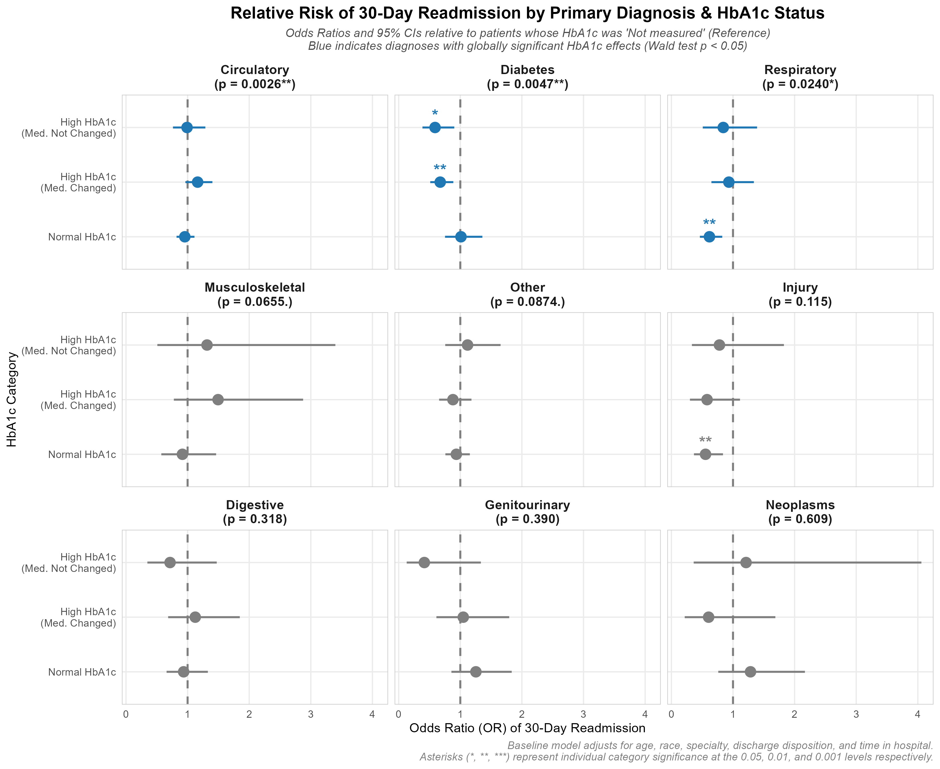
To resolve these visual scaling issues, I developed a faceted forest plot of Odds Ratios (OR) compared directly to the untested reference group (Not measured) within each diagnosis:

Dynamic Global & Individual Testing
- Global 3-df Wald test p-values are calculated using
car::linearHypothesis()and printed in the facet headers. - Significant panels (p < 0.05) are painted Blue, while non-significant ones are Grey.
- Individual category significance stars are plotted directly above the points.
Technical Insight: Understanding the Global 3-df Wald Test
When evaluating multi-categorical variables like hba1c_group (which has 4 levels: Not measured as reference, Normal, High, changed, and High, not changed), checking individual category p-values separately increases the risk of Type I error (false positives). To resolve this, we use a joint hypothesis test—the Wald test—to evaluate if the variable has a significant effect globally.
- Why 3 Degrees of Freedom (3-df)?: Since
hba1c_grouphas 4 levels, the regression model estimates 3 distinct dummy coefficients. The Wald test jointly tests the null hypothesis that all 3 coefficients are simultaneously zero . Testing these 3 independent parameters yields a test statistic that follows a Chi-square distribution with exactly 3 degrees of freedom. - Testing Subgroup Interactions: For non-baseline diagnoses (e.g., Circulatory), the Wald test evaluates whether the 3 diagnosis-specific interaction terms:
They are simultaneously zero. This verifies whether the HbA1c effect for that particular diagnosis is statistically different from the baseline Diabetes group.
Technical Insight: Standard Error Calculation with Covariance Matrix
Because of the primary diagnosis $\times$ HbA1c interaction terms in the final model, the log-Odds Ratio for non-reference diagnoses is a linear combination of coefficients: . I calculate the standard error utilizing the covariance matrix:
# Covariance-based standard error calculation in R (visualization_improved.R)log_or <- coefs[coef_hba1c] + coefs[coef_interaction]# Var(A + B) = Var(A) + Var(B) + 2 * Cov(A, B)var_log_or <- vc_mat[coef_hba1c, coef_hba1c] + vc_mat[coef_interaction, coef_interaction] + 2 * vc_mat[coef_hba1c, coef_interaction]se_log_or <- sqrt(var_log_or)odds_ratio <- exp(log_or)ci_lower <- exp(log_or - 1.96 * se_log_or)ci_upper <- exp(log_or + 1.96 * se_log_or)# Individual two-tailed p-valueindiv_p <- 2 * pnorm(-abs(log_or / se_log_or))
Findings & The Statistical Paradox
My modernized forest plot uncovers a fascinating statistical paradox: global interaction significance does not always align with individual category significance.
1. The Circulatory Paradox (Globally Significant, Individually Non-Significant)
- Global Test: (Blue Panel)
- Individual Odds Ratios:
- High, changed:
- High, not changed:
- Normal:
- The Paradox: Even though Circulatory is globally significant, not a single individual HbA1c category is statistically different from the untested reference group (all 95% CIs cross 1.0). The global significance is driven entirely by the comparison to the Diabetes baseline: Circulatory patients’ readmission risk trends upward for high HbA1c, while Diabetes trends downward.
2. The Injury Discovery (Globally Non-Significant, Individually Significant)
- Global Test: (Grey Panel)
- Individual Category Estimates:
- Normal: (Highly Significant)
- The Story: Although the overall trend for Injury does not differ enough from baseline to pass global interaction significance, Injury patients who received an HbA1c test that came back Normal had a 45% lower risk of readmission () than those who were not tested.
The injury diagnosis group has a total of 4,649 patients, while the untested reference category (Not measured) contains 4,117 patients (88.56%). This high proportion of untested patients causes a disproportionality in the data (leaving very few tested cases), which can lead to less reliable statistical estimates for the tested subgroups. Consequently, this finding needs further investigation to confirm its validity.
3. The Diabetes Story (Globally and Individually Significant)
- Global Test: (Blue Panel)
- Individual Category Estimates:
- High, changed: (Highly Significant)
- High, not changed: (Significant)
- Normal: (Not significant)
- The Story: For primary Diabetes admissions, measuring HbA1c is associated with a significant reduction in readmissions only if the result is high (prompting active medication changes). Testing normal HbA1c does not change readmission rates.
4. The Respiratory Story (Globally and Individually Significant)
- Global Test: (Blue Panel)
- Individual Category Estimates:
- Normal: (Highly Significant)
- The Story: For Respiratory patients, the reduction in readmission is isolated entirely to the Normal HbA1c group (), while high HbA1c groups show no significant benefit.
Discussions
Clinical Nuances & Cohort Context
- Cohort Selection: Out of over 100,000 raw clinical encounters, only 69,987 records met the strict inclusion criteria. This filtering was necessary to focus on independent, non-procedure-based encounters for patients surviving their hospital stay.
- Low Historical Prevalence: In this historical cohort (1999–2008), the HbA1c test was ordered in only 18.4% of inpatient stays. This indicates that inpatient screening was historically underutilized. However, the average length of stay of 4.27 days represents a highly sufficient clinical window for performing the test and receiving results.
- EHR Data Limitations: It is possible that HbA1c tests were evaluated in practice but not documented in the electronic health record (EHR) database, or that practitioners had access to other unrecorded blood glucose metrics (e.g., fingerstick logs) that guided medication adjustments. Additionally, standard guidelines recommending the discontinuation of outpatient diabetic medications upon admission were only adopted late in the study period.
- Modern Context (The HITECH Act): Since the 2009 HITECH Act and the introduction of hospital quality incentives (e.g., HEDIS/CMS measures), modern inpatient HbA1c screening has skyrocketed to exceed 70–80% for diabetic inpatients, representing a massive shift in standards of care compared to the historical baseline.
- Glycemic Attention & Readmission: With respect to readmission rates, simply measuring HbA1c is associated with a lower rate of readmission in individuals with diabetes as a primary diagnosis, whereas respiratory and circulatory diseases as primary diagnoses are not. This suggests that greater attention to diabetes care during hospitalization (specifically for these high-risk individuals) can have a significant clinical impact on readmission outcomes.
Methodological Limitations
- Retrospective, Nonrandomized Design: Unlike a randomized clinical trial (RCT), this study relies on a retrospective observational database. Because clinicians do not order HbA1c tests randomly, tested patients likely had different baseline risks, introducing selection bias.
- Association vs. Causal Inference: Consequently, this regression analysis reveals statistical associations rather than direct cause-and-effect relationships. However, these associations provide a strong empirical basis for developing and testing structured clinical protocols.
Proposed Future Improvements
To overcome the inherent limitations of the 2014 study design and nested logistic regression, three major methodological extensions are proposed:
1. Causal Inference (Selection Bias & Propensity Score Matching)
Because this is a retrospective clinical database and not a randomized controlled trial, physicians do not order HbA1c tests randomly. Sicker patients or those showing poor glycemic control are tested more frequently, introducing selection bias.
- Proposed Enhancement: Implementing Propensity Score Matching (PSM) to match tested and untested patients with identical baseline covariates (demographics, comorbidities, time in hospital) will allow us to isolate the true causal effect of inpatient HbA1c testing on readmissions.
2. Machine Learning & Model Interpretability
Logistic regression assumes linear log-odds relations and struggles to capture complex, high-order interactions without manual specification.
- Proposed Enhancement: Training a tree-based machine learning model (such as XGBoost) and generating SHAP (Shapley Additive exPlanations) values will allow us to capture non-linear risks and identify the exact contribution of medications and comorbidity scores to readmission.
3. Survival Analysis (Time-to-Event Modeling)
Analyzing readmissions as a binary 30-day flag ignores the timing of the readmission and treats a patient readmitted on day 31 identically to one who was never readmitted.
- Proposed Enhancement: Transitioning to a Cox Proportional Hazards model allows us to analyze the time-to-event outcome. This treats patients who were never readmitted (or discharged safely beyond the observation window) as right-censored, preserving temporal detail and statistical power.
Conclusion
- Clinical Value of HbA1c Screening: Inpatient HbA1c measurement is a highly valuable predictor of 30-day readmission rates, particularly for patients admitted with a primary diagnosis of Diabetes.
- Reducing Rates & Healthcare Costs: By identifying poorly controlled glycemic status during hospital stays and prompting active treatment adjustments, inpatient screening serves as a powerful catalyst for reducing costly readmissions and improving diabetic patient care.
- Empirical Foundation: Although the study is limited by its retrospective, nonrandomized design, the findings provide a strong empirical foundation for developing hospital protocols to test this clinical hypothesis directly.
Scripts
Full scripts are available at 
preprocess.R: Data filtering, ICD-9 diagnosis mapping, and cohort cleaning.analysis.R: Fits nested logistic regression models and calculates ANOVA deviance tables.visualization.R: Replicates the original paper’s Figures 1, 2, and 3.visualization_improved.R: The modernized visualization script implementing Wald tests and the faceted forest plot.run_pipeline.R: Master orchestrator script that runs the entire pipeline end-to-end and outputs a verification summary report.
Thank you for making it this far! This project demonstrates the power of transforming complex raw tabulations into granular, actionable clinical insights. Stay tuned for my next data science project!
Leave a Reply